In a previous blog post, we talked about how a sliding window framework can be used to create realistic datasets for training models. In that post, we talked about using a lookback window, but not how to decide on the size of that window. In this post, we’ll describe how to choose the appropriate window size for your dataset, and what tradeoffs you need to consider when making that choice.
What is Cohort Analysis?
The way Syntasa evaluates different choices for lookback windows bears resemblance to cohort analysis, a behavioral analysis technique commonly used in the digital ad space. In cohort analysis, a group of users with a similar attribute is chosen (that’s the “cohort”) and they are followed over a period of time. For example, a cohort could be all of the users who created an account on your website on a given day. Their defining attribute is the day that they created their account. The cohort analysis would then look at how many users from that original cohort came back to your website on each subsequent day.
Cohort analyses can be useful for determining metrics such as retention rate.
Using Cohort Analysis to Look Back in Time
Syntasa transformed traditional cohort analysis to make it usable as a tool for analyzing the effectiveness of lookback windows. The basic idea is the same: a group of users who share a common attribute are followed over time.
However, instead of following users forward in time, we are tracking users back in time. So our “cohort” in this kind of window analysis might be all of the users who made a purchase on a given day. Then, instead of following those users through their future activity, we look at the activity that led up to the purchase and search for the first time that each user in the cohort was seen.
By getting a count of the number of users first seen on each preceding day, we can then get an idea of how long a typical purchase journey is in the dataset.
Ideally, you would be able to follow the entire cohort all the way back to their very first visit. In practice, however, you need to strike a balance between having a window large enough to capture meaningful activity and having a window small enough to be feasible in terms of both cost and computation.
Seeing the Analysis in Action
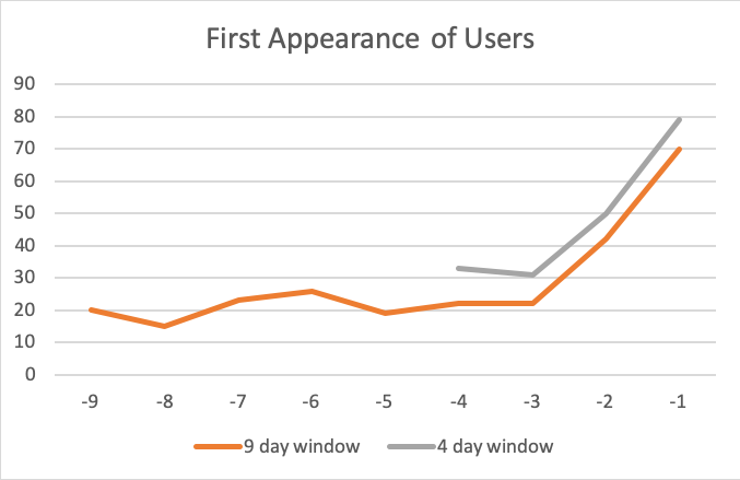
One method for finding that middle ground (and the one that Syntasa most often uses) is to find a window that minimizes the “spike” of users that will be seen at the end of a short window. Such a spike can be seen in the plot below, showing two windows from the same cohort of users who made a purchase on a consumer electronics website.
The plot shows the number of users (y-axis) that were first seen x days (x-axis) before their purchase. At the end of each window there is a slight uptick in users (the “spike”), indicating that some users would have fallen farther out on the graph, had the window been larger.
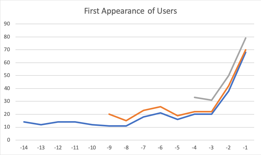
In general, the larger the window, the smaller the spike you’ll see. A 14-day window (the blue line on the plot below) further reduces the spike to the point where it’s barely noticeable. This indicates that your window is capturing a more complete image of your users’ journeys.
Analyzing Another Dataset
What about other datasets from other industries?
Is 14 days a generalizable window?
Let’s examine a cohort of users who made a purchase in the travel industry on a given day.
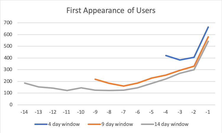
At 14 days we still see a noticeable rise in users at the end of the window.
Let’s try a larger window.
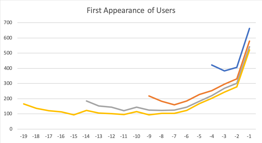
This shows that even with a 19-day window (yellow line), there is still a noticeable spike, indicating that an even larger window might be necessary. However, at 19 days you need to start thinking about how increasing your window size will affect resource use. Depending on the size of your dataset, trying to create features with these 19 days of data could start to creep past GB and move into the TB range.
Takeaways
By running this modified cohort analysis with various window sizes, you can evaluate what you might be gaining or losing with each one. A large window may capture a more accurate picture of your users’ journey than a smaller window, but that accuracy comes with a cost. The right balance depends heavily on your goals and your budget, and needs to be evaluated with both in mind.
Additionally, we showed that customers behave differently in different environments, necessitating a window that reflects their varying journeys. An analysis run on a previous dataset may not apply to your current dataset. And, even within a dataset, different groups of users may behave differently than others. Finding how or whether different groups behave differently may require separate analyses.
By running this modified cohort analysis with various window sizes, you can evaluate what you might be gaining or losing with each one.